Beam Blockage Calculation using a DEM
Here, we derive (partial) beam-blockage (PBB) from a Digital Elevation Model (DEM).
We require - the local radar setup (sitecoords, number of rays, number of bins, antenna elevation, beamwidth, and the range resolution); - a DEM with a adequate resolution.
Here we use pre-processed data from the GTOPO30 and SRTM missions.
In [1]:
import wradlib as wrl
import matplotlib.pyplot as pl
import matplotlib as mpl
import warnings
warnings.filterwarnings('ignore')
try:
    get_ipython().magic("matplotlib inline")
except:
    pl.ion()
import numpy as np
Setup for Bonn radar
First, we need to define some radar specifications (here: University of Bonn).
In [2]:
sitecoords = (7.071663, 50.73052, 99.5)
nrays = 360 # number of rays
nbins = 1000 # number of range bins
el = 1.0 # vertical antenna pointing angle (deg)
bw = 1.0 # half power beam width (deg)
range_res = 100. # range resolution (meters)
Create the range, azimuth, and beamradius arrays.
In [3]:
r = np.arange(nbins) * range_res
beamradius = wrl.util.half_power_radius(r, bw)
We use
to calculate the spherical coordinates of the bin centroids and their longitude, latitude and altitude.
In [4]:
coord = wrl.georef.sweep_centroids(nrays, range_res, nbins, el)
coords = wrl.georef.spherical_to_proj(coord[..., 0],
                                      np.degrees(coord[..., 1]),
                                      coord[..., 2], sitecoords)
lon = coords[..., 0]
lat = coords[..., 1]
alt = coords[..., 2]
In [5]:
polcoords = coords[..., :2]
print("lon,lat,alt:", coords.shape)
lon,lat,alt: (360, 1000, 3)
In [6]:
rlimits = (lon.min(), lat.min(), lon.max(), lat.max())
print("Radar bounding box:\n\t%.2f\n%.2f             %.2f\n\t%.2f" %
      (lat.max(), lon.min(), lon.max(), lat.min()))
Radar bounding box:
        51.63
5.66             8.49
        49.83
Preprocessing the digitial elevation model
- Read the DEM from a
geotifffile (inWRADLIB_DATA); - clip the region inside the bounding box;
- map the DEM values to the polar grid points.
Note: You can choose between the coarser resolution bonn_gtopo.tif
(from GTOPO30) and the finer resolution bonn_new.tif (from the SRTM
mission).
The DEM raster data is opened via wradlib.io.open_raster and extracted via wradlib.georef.extract_raster_dataset.
In [7]:
#rasterfile = wrl.util.get_wradlib_data_file('geo/bonn_gtopo.tif')
rasterfile = wrl.util.get_wradlib_data_file('geo/bonn_new.tif')

ds = wrl.io.open_raster(rasterfile)
rastervalues, rastercoords, proj = wrl.georef.extract_raster_dataset(ds, nodata=-32768.)

# Clip the region inside our bounding box
ind = wrl.util.find_bbox_indices(rastercoords, rlimits)
rastercoords = rastercoords[ind[1]:ind[3], ind[0]:ind[2], ...]
rastervalues = rastervalues[ind[1]:ind[3], ind[0]:ind[2]]

# Map rastervalues to polar grid points
polarvalues = wrl.ipol.cart_to_irregular_spline(rastercoords, rastervalues,
                                             polcoords, order=3,
                                             prefilter=False)
Calculate Beam-Blockage
Now we can finally apply the wradlib.qual.beam_block_frac function to calculate the PBB.
In [8]:
PBB = wrl.qual.beam_block_frac(polarvalues, alt, beamradius)
PBB = np.ma.masked_invalid(PBB)
print(PBB.shape)
(360, 1000)
So far, we calculated the fraction of beam blockage for each bin.
But we need to into account that the radar signal travels along a beam. Cumulative beam blockage (CBB) in one bin along a beam will always be at least as high as the maximum PBB of the preceeding bins (see wradlib.qual.cum_beam_block_frac)
In [9]:
CBB = wrl.qual.cum_beam_block_frac(PBB)
print(CBB.shape)
(360, 1000)
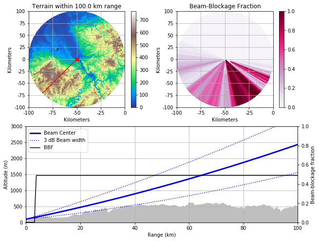
Visualize Beamblockage
Now we visualize - the average terrain altitude per radar bin - a beam blockage map - interaction with terrain along a single beam
In [10]:
# just a little helper function to style x and y axes of our maps
def annotate_map(ax, cm=None, title=""):
    ticks = (ax.get_xticks()/1000).astype(np.int)
    ax.set_xticklabels(ticks)
    ticks = (ax.get_yticks()/1000).astype(np.int)
    ax.set_yticklabels(ticks)
    ax.set_xlabel("Kilometers")
    ax.set_ylabel("Kilometers")
    if not cm is None:
        pl.colorbar(cm, ax=ax)
    if not title=="":
        ax.set_title(title)
    ax.grid()
In [11]:
fig = pl.figure(figsize=(10, 8))

# create subplots
ax1 = pl.subplot2grid((2, 2), (0, 0))
ax2 = pl.subplot2grid((2, 2), (0, 1))
ax3 = pl.subplot2grid((2, 2), (1, 0), colspan=2, rowspan=1)

# azimuth angle
angle = 225

# Plot terrain (on ax1)
ax1, dem = wrl.vis.plot_ppi(polarvalues,
                            ax=ax1, r=r,
                            az=np.degrees(coord[:,0,1]),
                            cmap=mpl.cm.terrain, vmin=0.)
ax1.plot([0,np.sin(np.radians(angle))*1e5],
         [0,np.cos(np.radians(angle))*1e5],"r-")
ax1.plot(sitecoords[0], sitecoords[1], 'ro')
annotate_map(ax1, dem, 'Terrain within {0} km range'.format(np.max(r / 1000.) + 0.1))

# Plot CBB (on ax2)
ax2, cbb = wrl.vis.plot_ppi(CBB, ax=ax2, r=r,
                            az=np.degrees(coord[:,0,1]),
                            cmap=mpl.cm.PuRd, vmin=0, vmax=1)
annotate_map(ax2, cbb, 'Beam-Blockage Fraction')

# Plot single ray terrain profile on ax3
bc, = ax3.plot(r / 1000., alt[angle, :], '-b',
               linewidth=3, label='Beam Center')
b3db, = ax3.plot(r / 1000., (alt[angle, :] + beamradius), ':b',
                 linewidth=1.5, label='3 dB Beam width')
ax3.plot(r / 1000., (alt[angle, :] - beamradius), ':b')
ax3.fill_between(r / 1000., 0.,
                 polarvalues[angle, :],
                 color='0.75')
ax3.set_xlim(0., np.max(r / 1000.) + 0.1)
ax3.set_ylim(0., 3000)
ax3.set_xlabel('Range (km)')
ax3.set_ylabel('Altitude (m)')
ax3.grid()

axb = ax3.twinx()
bbf, = axb.plot(r / 1000., CBB[angle, :], '-k',
                label='BBF')
axb.set_ylabel('Beam-blockage fraction')
axb.set_ylim(0., 1.)
axb.set_xlim(0., np.max(r / 1000.) + 0.1)


legend = ax3.legend((bc, b3db, bbf),
                    ('Beam Center', '3 dB Beam width', 'BBF'),
                    loc='upper left', fontsize=10)
Visualize Beam Propagation showing earth curvature
Now we visualize - interaction with terrain along a single beam
In this representation the earth curvature is shown. For this we assume the earth a sphere with exactly 6370000 m radius. This is needed to get the height ticks at nice position.
In [12]:
def height_formatter(x, pos):
    x = (x - 6370000) / 1000
    fmt_str = '{:g}'.format(x)
    return fmt_str

def range_formatter(x, pos):
    x = x / 1000.
    fmt_str = '{:g}'.format(x)
    return fmt_str
- The wradlib.vis.create_cg-function is facilitated to create the curved geometries.
- The actual data is plottet as (theta, range) on the parasite axis.
- Some tweaking is needed to get the final plot look nice.
In [13]:
fig = pl.figure(figsize=(10, 6))

cgax, caax, paax = wrl.vis.create_cg('RHI', fig, 111)

# azimuth angle
angle = 225

# fix grid_helper
er = 6370000
gh = cgax.get_grid_helper()
gh.grid_finder.grid_locator2._nbins=80
gh.grid_finder.grid_locator2._steps=[1,2,4,5,10]

# calculate beam_height and arc_distance for ke=1
# means line of sight
bhe = wrl.georef.bin_altitude(r, 0, sitecoords[2], re=er, ke=1.)
ade = wrl.georef.bin_distance(r, 0, sitecoords[2], re=er, ke=1.)
nn0 = np.zeros_like(r)
# for nice plotting we assume earth_radius = 6370000 m
ecp = nn0 + er
# theta (arc_distance sector angle)
thetap = - np.degrees(ade/er) + 90.0

# zero degree elevation with standard refraction
bh0 = wrl.georef.bin_altitude(r, 0, sitecoords[2], re=er)

# plot (ecp is earth surface normal null)
bes, = paax.plot(thetap, ecp, '-k', linewidth=3, label='Earth Surface NN')
bc, = paax.plot(thetap, ecp + alt[angle, :], '-b', linewidth=3, label='Beam Center')
bc0r, = paax.plot(thetap, ecp + bh0 + alt[angle, 0] , '-g', label='0 deg Refraction')
bc0n, = paax.plot(thetap, ecp + bhe + alt[angle, 0], '-r', label='0 deg line of sight')
b3db, = paax.plot(thetap, ecp + alt[angle, :]  + beamradius, ':b', label='+3 dB Beam width')
paax.plot(thetap, ecp + alt[angle, :] - beamradius, ':b', label='-3 dB Beam width')

# orography
paax.fill_between(thetap, ecp,
                  ecp + polarvalues[angle, :],
                  color='0.75')

# shape axes
cgax.set_xlim(0, np.max(ade))
cgax.set_ylim([ecp.min()-1000, ecp.max()+2500])
caax.grid(True, axis='x')
cgax.grid(True, axis='y')
cgax.axis['top'].toggle(all=False)
caax.yaxis.set_major_locator(mpl.ticker.MaxNLocator(steps=[1,2,4,5,10], nbins=20, prune='both'))
caax.xaxis.set_major_locator(mpl.ticker.MaxNLocator())
caax.yaxis.set_major_formatter(mpl.ticker.FuncFormatter(height_formatter))
caax.xaxis.set_major_formatter(mpl.ticker.FuncFormatter(range_formatter))

caax.set_xlabel('Range (km)')
caax.set_ylabel('Altitude (km)')

legend = paax.legend((bes, bc0n, bc0r, bc, b3db),
                    ('Earth Surface NN', '0 deg line of sight', '0 deg std refraction', 'Beam Center', '3 dB Beam width'),
                    loc='upper left', fontsize=10)

Go back to Read DEM Raster Data, change the rasterfile to use the other resolution DEM and process again.